Kinematic

Prior part design (or after for assembly), we may want to see how what we are making should behave. We use then a Kinematic, using the current engineering conventions. In the same spirit as for the primitives, the solvekin function solves the joints constraints.

from madcad import *
# We define the solids, they intrinsically have nothing particular
base = Solid()
s1 = Solid()
s2 = Solid()
s3 = Solid()
s4 = Solid()
s5 = Solid()
wrist = Solid(name='wrist') # give it a fancy name

# The joints defines the kinematic.
# This is a 6 DoF (degrees of freedom) robot arm
csts = [
    Pivot(base, s1, (O, Z)),  # (1)!
    Pivot(s1, s2, (vec3(0, 0, 1), X), (O, X)),  # (2)!
    Pivot(s2, s3, (vec3(0, 0, 2), X), (O, X)),
    Pivot(s3, s4, (vec3(0, 0, 1), Z), (vec3(0, 0, -1), Z)),
    Pivot(s4, s5, (O, X)),
    Pivot(s5, wrist, (vec3(0, 0, 0.5), Z), (O, Z)),
]

# The kinematic is created with some
# fixed solids (they interact but they do not move)
kin = Kinematic(csts, fixed=[base])

# Solve the current position (not necessary
# if just need a display)
solvekin(csts)

show([kin])

1. Pivot using axis (O,Z) both in solid base and solid 1
2. Pivot using different axis coordinates in each solid

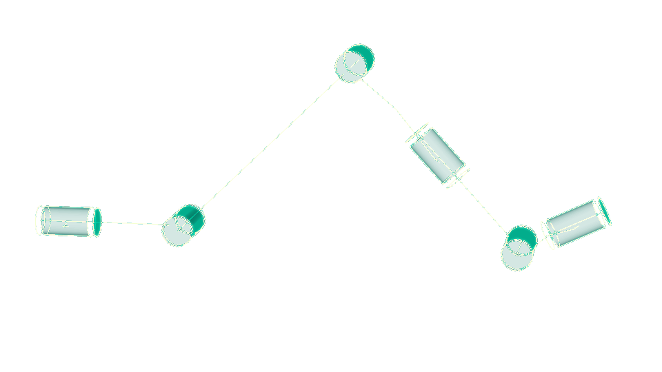
Kinematics are displayable as interactive objects the user can move. They also are useful to compute force distributions during the movements or movement trajectories or kinematic cycles ...